Understanding Quantum Optimization: A Beginner's Guide

How Quantum Computers Might Solve the World's Hardest Problems A simplified introduction to quantum optimization, QUBO formulations, and the mathematics behind breakthrough research from IBM Quantum

Optimization problems are ubiquitous in modern computing, from routing delivery vehicles to designing microchips. While classical computers have made tremendous progress in solving these problems, many remain intractable at scale. Quantum computers offer a fundamentally different approach that may unlock new capabilities for specific problem classes.

Imagine you’re planning a road trip to visit 10 different cities. You want to find the shortest possible route that visits each city exactly once and returns home. Sounds simple, right?

Here’s the catch: with just 10 cities, there are over 3.6 million possible routes to check! With 20 cities, that number jumps to over 2 quintillion (that’s 2 followed by 18 zeros). Even the fastest supercomputers would take forever to check every single possibility.

This is an optimization problem - finding the best solution from an enormous number of possibilities. And this is exactly what quantum computers might help us solve more efficiently.

This is the first in a series of technical articles exploring quantum optimization, based on recent research from IBM Quantum and the Quantum Optimization Working Group. We’ll build from foundational concepts to cutting-edge techniques, with rigorous mathematics and practical insights.

---

The Optimization Problem

Optimization in Your Daily Life

You solve optimization problems all the time without even thinking about it:

• Morning routine: What order should you shower, eat breakfast, and get dressed to save time?

• Grocery shopping: Which store gives you the best prices for everything on your list?

• Netflix: Which show should you watch to maximize your enjoyment?

• Parking: Where should you park to minimize walking distance?

In each case, you’re trying to find the “best” choice according to some criteria (time, money, happiness, effort).

General Form

An optimization problem seeks to find values of decision variables that minimize (or maximize) an objective function while satisfying constraints:

\( \begin{align}\text{minimize} \quad & f(\mathbf{x}) \\\text{subject to} \quad & g_i(\mathbf{x}) \leq 0, \quad i = 1, \ldots, m \\& h_j(\mathbf{x}) = 0, \quad j = 1, \ldots, p \\& \mathbf{x} \in \mathcal{X}\end{align} \)

Where:

\(\begin{aligned} &\mathbf{x} = (x_1, x_2, \ldots, x_n) \quad \text{is the vector of decision variables}, \\ &f: \mathbb{R}^n \rightarrow \mathbb{R} \quad \text{is the objective function}, \\ &g_i(\mathbf{x}) \leq 0, \quad i = 1, \ldots, m \quad \text{are the inequality constraints}, \\ &h_j(\mathbf{x}) = 0, \quad j = 1, \ldots, p \quad \text{are the equality constraints}, \\ &\mathcal{X} \subseteq \mathbb{R}^n \quad \text{defines the variable domain (e.g., } \mathbb{R}^n, \mathbb{Z}^n, \{0,1\}^n \text{)}. \end{aligned}\)

The Three Parts of Every Optimization Problem

Every optimization problem has three ingredients:

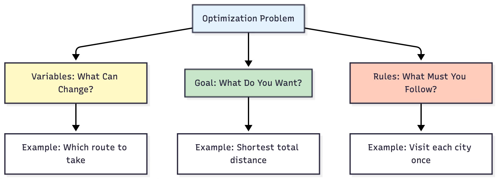
1. Variables (Things you can change)

• Think of these as the “knobs” you can turn

• Example: In the road trip, the order of cities you visit

2. Goal/Objective (What you’re trying to achieve)

• Usually “minimize” something bad (cost, time, distance)

• Or “maximize” something good (profit, happiness, efficiency)

• Example: Minimize total travel distance

3. Constraints (Rules you must follow)

• Limitations on what’s allowed

• Example: Must visit each city exactly once

Why Are These Problems So Hard?

Let’s look at how quickly the number of possibilities grows:

This is called exponential growth - the number of possibilities explodes as the problem gets bigger. Even if you could check 1 billion routes per second, checking all routes for 20 cities would take over 77 years!

Combinatorial Optimization

Quantum optimization research primarily focuses on combinatorial optimization, where variables are discrete:

\(\mathbf{x} \in \{0,1\}^n \quad \text{or} \quad \mathbf{x} \in \mathbb{Z}^n\)

Example: Traveling Salesperson Problem (TSP)

\(\begin{aligned} &\text{Given } n \text{ cities with distances } d_{ij} \text{ between cities } i \text{ and } j, \\ &\text{find the shortest tour visiting each city exactly once.} \\ &\\ &\text{Decision variables: } x_{ij} \in \{0,1\} \text{ where } x_{ij} = 1 \text{ if edge } (i,j) \text{ is in the tour.} \end{aligned}\)

\(\begin{align} \text{minimize} \quad & \sum_{i=1}^{n} \sum_{j=1}^{n} d_{ij} x_{ij} \\ \text{subject to} \quad & \sum_{j=1}^{n} x_{ij} = 1, \quad \forall i \quad \text{(leave each city once)} \\ & \sum_{i=1}^{n} x_{ij} = 1, \quad \forall j \quad \text{(enter each city once)} \\ & \text{no subtours} \end{align}\)

How Computers Solve These Problems

Three Approaches

Computers use different strategies depending on the situation:

Approach 1: Check Everything (Brute Force)

• Look at every single possibility

• Guaranteed to find the best answer

• Problem: Takes way too long for big problems

Approach 2: Be Smart (Clever Algorithms)

• Use mathematical tricks to eliminate obviously bad solutions

• Much faster than checking everything

• Still struggles with very large problems

Approach 3: Get Close Enough (Approximation)

• Find a “pretty good” solution, not necessarily the best

• Fast and practical

• Might miss the absolute best answer, but that’s okay

Real-world secret: Most companies don’t need the perfect solution - they need a good enough solution quickly. A delivery company is happy with a route that’s 5% longer than optimal if they can find it in 10 seconds instead of 10 hours.

Where Quantum Computers Fit In

Quantum computers offer a fourth approach:

Approach 4: Quantum Exploration

• Use quantum physics properties to explore many possibilities simultaneously

• Not magic - still can’t check everything instantly

• Might find good solutions faster for certain types of problems

Think of it like this:

• Classical computer: Checks paths one at a time, like walking through a maze

• Quantum computer: Can “sense” multiple paths at once, like having a bird’s-eye view

Translating Problems for Quantum Computers

Why Translation Matters

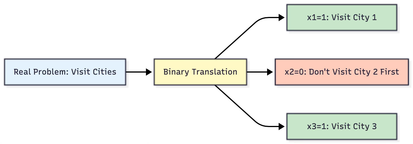
Quantum computers don’t understand road trips, city names, or distances. They only understand quantum bits (qubits) and quantum physics. So we need to translate our everyday problems into a language quantum computers can work with.

It’s like translating a story from English to French - the meaning stays the same, but the words change.

Binary Variables: The Quantum Language

Quantum computers work best with binary variables - things that are either 0 or 1, yes or no, true or false.

Examples of binary decisions:

• Should I include this item in my backpack? (yes=1, no=0)

• Is this person on Team A or Team B? (A=0, B=1)

• Is this light on or off? (off=0, on=1)

Why binary? Each quantum bit (qubit) can represent a 0 or 1, so binary problems map naturally to quantum hardware.

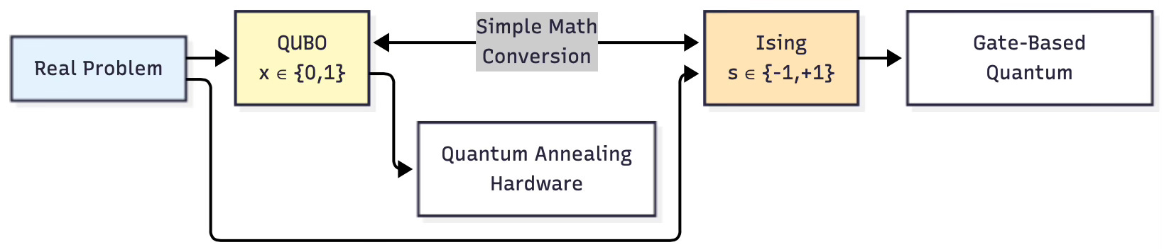
Two Ways to Speak Quantum: QUBO and Ising

There are two main “dialects” for translating problems to quantum computers. Think of them as two dialects of the same language—different notation, same meaning.

QUBO (Quadratic Unconstrained Binary Optimization)

What it means:

• Quadratic: Variables multiplied together (x₁ × x₂)

• Unconstrained: No explicit rules (we’ll hide rules in the cost)

• Binary: Variables are 0 or 1

• Optimization: Finding the best solution

Simple example: Imagine you want to choose between 3 items for your backpack, but some items work well together (rewards) and others don’t (penalties).

Variables: x₁, x₂, x₃ (each is 0 or 1)

Cost function (we want to minimize this):

Cost = -5x₁ - 3x₂ - 4x₃ + 2x₁x₂ + 3x₁x₃ + 1x₂x₃

\(C = -5x_1 - 3x_2 - 4x_3 + 2x_1 x_2 + 3x_1 x_3 + 1x_2 x_3\)

What this means in English:

• Item 1 saves you 5 (negative means good!)

• Item 2 saves you 3

• Item 3 saves you 4

• But if you take items 1 AND 2 together, you lose 2 (they don’t fit well)

• If you take items 1 AND 3 together, you lose 3

• If you take items 2 AND 3 together, you lose 1

Goal: Find which combination of items (0s and 1s) makes the cost as low as possible.

\(\min_{\mathbf{x} \in \{0,1\}^n} f(\mathbf{x}) = \mathbf{x}^T Q \mathbf{x} = \sum_{i=1}^{n} \sum_{j=1}^{n} Q_{ij} x_i x_j\)

Ising Model (The Physics Version)

What it means:

• Originally from physics (modeling magnets)

• Uses “spins” that are +1 or -1 (instead of 0 or 1)

• Think of magnets that can point up (+1) or down (-1)

Why different from QUBO? Just a different way to represent the same thing. Like measuring temperature in Celsius vs. Fahrenheit - same temperature, different numbers.

Simple example: Four people (spins) can either “point up” (+1) or “point down” (-1). Friends want to point in opposite directions (to keep things interesting).

Energy function (we want to minimize this):

Energy = -(s₁ × s₂) - (s₂ × s₃) - (s₃ × s₄) - (s₄ × s₁)

What this means in English:

• When person 1 and person 2 point opposite ways, we get reward (energy goes down)

• When they point the same way, we get penalty (energy goes up)

• Same for all friend pairs

Goal: Find which direction each person should point to minimize total energy.

\(\begin{aligned} H(\mathbf{s}) = \sum_{i < j} J_{ij} s_i s_j + \sum_{i=1}^{n} h_i s_i \\ \\ \text{Where} \ s_i \in \{-1, +1\} \end{aligned}\)

Converting Between QUBO and Ising

These two formulations are equivalent - you can convert between them with simple algebra.

The conversion formula:

If QUBO uses x (where x = 0 or 1), and Ising uses s (where s = -1 or +1):

s = 2x - 1    (QUBO to Ising)
x = (s + 1)/2  (Ising to QUBO)

Example:

• If x = 0, then s = 2(0) - 1 = -1

• If x = 1, then s = 2(1) - 1 = +1

\(s_i = 2x_i - 1 \quad \Leftrightarrow \quad x_i = \frac{s_i + 1}{2}\)

Why two formats?

• QUBO is easier for business problems (yes/no decisions)

• Ising is more natural for quantum physics

• Quantum computers can use either one

A Complete Example: The MaxCut Problem

Let’s walk through a real problem step-by-step to see how all this works.

The Problem in Plain English

Scenario: You have 4 friends at a party. Some pairs of friends have met before, some haven’t. You want to divide them into two groups (Group A and Group B) to maximize “interesting” conversations - where people from different groups meet for the first time.

The Graph:

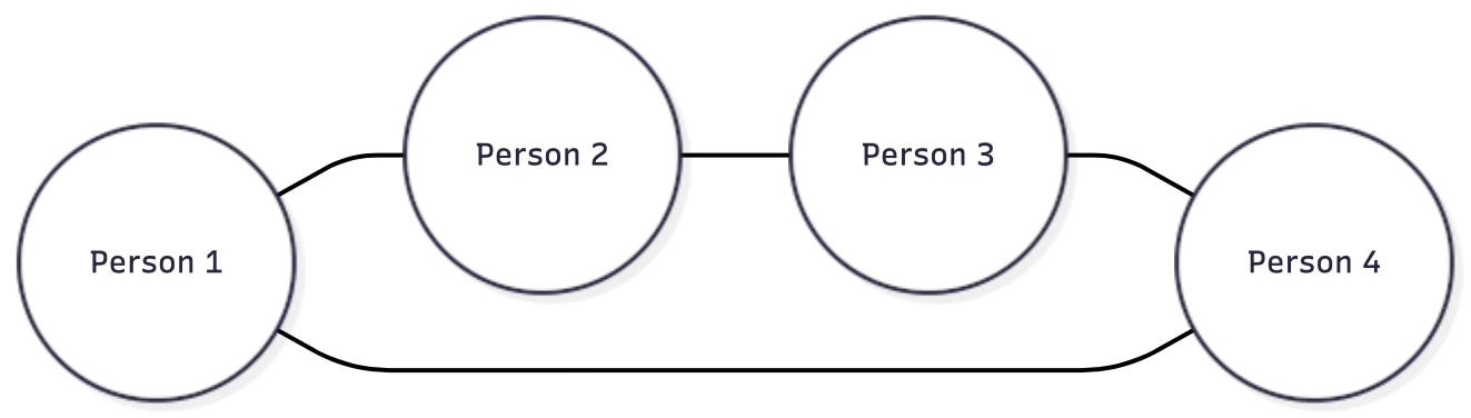
The lines show who has met before. You want as many lines as possible connecting Group A to Group B.

Setting Up Variables

We need a variable for each person:

• x₁ = 0 means Person 1 goes to Group A, x₁ = 1 means Group B

• x₂ for Person 2

• x₃ for Person 3

• x₄ for Person 4

Counting “Cuts” (Lines Between Groups)

For each pair of friends (each line), we want them in different groups.

The math trick:

• If x₁ = 0 and x₂ = 0 (both in Group A): x₁ + x₂ - 2x₁x₂ = 0 + 0 - 0 = 0 (not cut)

• If x₁ = 0 and x₂ = 1 (different groups): x₁ + x₂ - 2x₁x₂ = 0 + 1 - 0 = 1 (cut!)

• If x₁ = 1 and x₂ = 0 (different groups): x₁ + x₂ - 2x₁x₂ = 1 + 0 - 0 = 1 (cut!)

• If x₁ = 1 and x₂ = 1 (both in Group B): x₁ + x₂ - 2x₁x₂ = 1 + 1 - 2 = 0 (not cut)

Pattern: The formula x₁ + x₂ - 2x₁x₂ equals 1 when people are in different groups, 0 when in same group.

The Complete Cost Function

To maximize cuts, we want to maximize:

Total Cuts = (x₁ + x₂ - 2x₁x₂) + (x₂ + x₃ - 2x₂x₃) + (x₃ + x₄ - 2x₃x₄) + (x₄ + x₁ - 2x₄x₁)

Since computers minimize (not maximize), we flip the sign:

Cost = -[(x₁ + x₂ - 2x₁x₂) + (x₂ + x₃ - 2x₂x₃) + (x₃ + x₄ - 2x₃x₄) + (x₄ + x₁ - 2x₄x₁)]

\(\min_{\mathbf{x}} f(\mathbf{x}) = -\sum_{(i,j) \in E} (x_i + x_j - 2x_i x_j)\)

The lines show who has met before. You want as many lines as possible connecting Group A to Group B.

Testing a solution: Let’s try x₁=0, x₂=1, x₃=0, x₄=1 (alternating groups).

\(\begin{align} \text{Edge }(1,2): & \quad 0 + 1 - 2(0)(1) = 1 \quad \checkmark \\ \text{Edge }(2,3): & \quad 1 + 0 - 2(1)(0) = 1 \quad \checkmark \\ \text{Edge }(3,4): & \quad 0 + 1 - 2(0)(1) = 1 \quad \checkmark \\ \text{Edge }(4,1): & \quad 1 + 0 - 2(1)(0) = 1 \quad \checkmark \end{align}\)

All four edges are cut! The total number of cuts is:

\(\text{Total cuts} = 4, \quad \text{Cost} = -4\)

This is optimal—we cannot cut more than 4 edges in this graph.

In Ising format, using spins s_i ∈ {-1, +1}:

\(H_{\text{MaxCut}} = -(s_1s_2 + s_2s_3 + s_3s_4 + s_4s_1)\)

When spins point opposite directions (different groups), the product s_i s_j = -1, and the negative sign makes energy more negative (better). For quantum computers, we write this using Pauli Z operators:

\(H_{\text{MaxCut}} = -\sum_{(i,j) \in E} Z_i Z_j\)

Handling Constraints: The Penalty Method

Real-world problems have rules: budgets can’t be exceeded, every task must be assigned, resources are limited. But QUBO is “unconstrained”—no explicit rules allowed. How do we enforce them?

The solution is elegant: add penalties to the cost function. When a solution violates a rule, we add a large cost, making that solution unattractive.

The general penalty function is:

\(f_{\text{penalty}}(\mathbf{x}) = f(\mathbf{x}) + \lambda \cdot [g(\mathbf{x})]^2\)

where λ (lambda) is the penalty coefficient and g(x) = 0 when the constraint is satisfied.

Example: Choose exactly 2 items from 3 options.

Variables: x₁, x₂, x₃ (each 0 or 1)
Constraint: x₁ + x₂ + x₃ = 2
Original objective: f = 5x₁ + 3x₂ + 4x₃

Add penalty:

\(f_{\text{total}}(\mathbf{x}) = (5x_1 + 3x_2 + 4x_3) + \lambda(x_1 + x_2 + x_3 - 2)^2\)

When expanded, this becomes:

\(\begin{align} (x_1 + x_2 + x_3 - 2)^2 = &\, x_1 + x_2 + x_3 \\ &+ 2x_1x_2 + 2x_1x_3 + 2x_2x_3 \\ &- 4x_1 - 4x_2 - 4x_3 + 4 \end{align}\)

(We used the property that x² = x for binary variables.)

If you pick 2 items: (2-2)² = 0, penalty = 0 ✓
If you pick 3 items: (3-2)² = 1, penalty = λ ✗ Very expensive!

The penalty coefficient λ must be large enough to enforce the rule but not so large it causes numerical problems. A good rule of thumb:

\(\lambda \geq \frac{\max_{\mathbf{x}} |f(\mathbf{x})|}{\min_{\mathbf{x} : g(\mathbf{x}) \neq 0} [g(\mathbf{x})]^2}\)

Typically, λ values between 10 and 1000 work well in practice.

How Quantum Computers Approach Optimization

Classical computers check solutions sequentially or use clever tricks to prune obviously bad options. Quantum computers take a fundamentally different approach using superposition and interference.

Classical approach: Walk through a maze one path at a time, keeping track of the best route found.

Quantum approach: Represent all paths simultaneously in superposition, then use quantum interference to amplify good paths and suppress bad ones. After measurement, good solutions appear more frequently.

The quantum state representing solutions looks like:

\(|\psi\rangle = \sum_{\mathbf{x} \in \{0,1\}^n} \alpha_{\mathbf{x}} |\mathbf{x}\rangle\)

where α_x are complex probability amplitudes. These amplitudes must satisfy the normalization condition:

\(\sum_{\mathbf{x} \in \{0,1\}^n} |\alpha_{\mathbf{x}}|^2 = 1\)

When measured, solution x appears with probability:

\(P(\mathbf{x}) = |\alpha_{\mathbf{x}}|^2\)

The quantum algorithm manipulates these amplitudes to make good solutions more likely.

This doesn’t mean quantum computers “check all solutions instantly”—that’s impossible due to fundamental physics. Instead, they explore the solution space differently, potentially finding good solutions faster for certain problem structures.

The optimization problem is encoded as a quantum Hamiltonian (energy function):

\(H_C = \sum_{\mathbf{x} \in \{0,1\}^n} f(\mathbf{x}) |\mathbf{x}\rangle\langle\mathbf{x}|\)

Or in Ising form:

\(H_C = \sum_{i<j} J_{ij} Z_i Z_j + \sum_{i=1}^{n} h_i Z_i\)

The goal is to find the ground state (lowest energy state):

\(H_C |\psi_{\text{opt}}\rangle = E_{\text{min}} |\psi_{\text{opt}}\rangle\)

The energy of any state is given by the expectation value:

\(E = \langle \psi | H_C | \psi \rangle = \sum_{\mathbf{x}} P(\mathbf{x}) \cdot f(\mathbf{x})\)

From Theory to Practice: The Current State

Recent research from IBM Quantum, Los Alamos National Laboratory, and the University of Basel has demonstrated significant progress. A breakthrough technique called CVaR (Conditional Value at Risk) helps quantum computers overcome hardware noise by focusing on the best measurement outcomes.

CVaR is defined as:

\(\text{CVaR}_\alpha(H) = \frac{1}{\lceil \alpha N \rceil} \sum_{i=1}^{\lceil \alpha N \rceil} H_{(i)}\)

where H_(1) ≤ H_(2) ≤ ... ≤ H_(N) are sorted costs, and α ∈ [0,1] is the confidence level. Instead of averaging all samples (traditional expectation value), CVaR averages only the best α fraction of samples.

The theoretical guarantee is remarkable:

\(\text{CVaR}_\alpha(H_{\text{noisy}}) \leq \langle H \rangle_{\text{ideal}} + \epsilon(\alpha, \delta, N)\)

The error term scales as:

\( \epsilon(\alpha, \delta, N) = O\left(\frac{\|H\|}{\sqrt{\alpha N}} \log(1/\delta)\right)\)

This provides provable bounds on solution quality with only polynomial sampling overhead—a dramatic improvement over previous error mitigation methods that required exponential resources.

The Quantum Optimization Working Group’s Nature Reviews Physics white paper outlines both challenges and opportunities. Key insights include:

Current Reality: Quantum computers with 100-1000 qubits exist but remain noisy and error-prone. For most problems, classical computers still win.

Promise: For specific problem structures—dense coupling, high connectivity, complex constraints—quantum approaches might offer advantages, especially in the 50-500 variable range where classical methods struggle but problems are small enough for current quantum hardware.

Path Forward: The future likely involves hybrid quantum-classical algorithms where quantum processors handle the hardest computational steps while classical computers manage data, parameters, and post-processing.

---

Why This Matters

Optimization problems permeate modern society. Even modest improvements can yield enormous value:

• Logistics: A 5% improvement in delivery routing saves millions in fuel costs

• Finance: Better portfolio optimization affects trillions in managed assets

• Healthcare: Optimized hospital scheduling improves patient outcomes

• Energy: Efficient grid management reduces waste and costs

Performance is measured by the approximation ratio:

\(r = \frac{C_{\text{found}}}{C_{\text{optimal}}}\)

For minimization problems, we want r close to 1. The time to find a solution with 99% confidence is:

\(\text{TTS} = t_{\text{single}} \cdot \frac{\ln(1 - 0.99)}{\ln(1 - p_{\text{success}})}\)

Quantum optimization won’t replace classical methods entirely. Instead, it offers a new tool for problems where classical approaches hit computational walls. As quantum hardware improves and algorithms become more sophisticated, we may see practical quantum advantages emerge for specific, high-value problem classes.

The journey from theoretical possibility to practical impact continues. With systematic benchmarking, honest comparisons against state-of-the-art classical methods, and continued algorithmic innovation, quantum optimization is moving from laboratory curiosity to potential industrial tool.

---

Conclusion

Quantum optimization represents a fascinating intersection of quantum physics, computer science, and operations research. While popular media sometimes overhypes quantum computing’s capabilities, rigorous research shows genuine potential for specific problem types.

The key mathematical frameworks—QUBO and Ising formulations—provide the bridge between real-world problems and quantum hardware. Techniques like penalty methods allow us to encode complex constraints, while breakthrough methods like CVaR help overcome current hardware limitations.

Understanding these foundations prepares us for the next phase: the quantum algorithms themselves (like QAOA), error mitigation techniques, and systematic benchmarking protocols that will determine where quantum computers truly excel.

The quantum optimization revolution won’t be instant or universal, but for certain hard problems, it may provide the computational edge that classical computers cannot match. As researchers continue pushing boundaries, the problems deemed “intractable” today might become solvable tomorrow.

---

Key Takeaways

• Optimization problems grow exponentially hard with size: 2^n possible solutions

• QUBO (0/1) and Ising (+1/-1) formats translate problems for quantum computers

• Constraints are encoded as penalties: f_total = f + λ(constraint)²

• Quantum computers use superposition to explore solutions differently

• CVaR provides polynomial-overhead error mitigation for noisy quantum hardware

• Current research shows promise for 50-500 variable problems with specific structures

• Hybrid quantum-classical approaches are likely the practical path forward